blog
/
research
Campaign-Level Incrementality: How to Scale the Right Campaign When Your MMM Only Sees Channel Level
Your MMM gives channel-level incrementality. Learn how to distribute it to campaign level without holdout tests.


Get a weekly dose of insightful people strategy content
Channel-level incrementality is identifiable from data. Campaign-level incrementality requires a transparent set of assumptions to be distributed from it.
Key Takeaways
MMMs measure incrementality at channel level, not campaign level — statistical power, multicollinearity and campaign churn make campaign-level causal measurement impossible with the same data.
You don't need holdout tests for every campaign. Rule B distributes the channel-level incremental revenue to campaigns using spend and attributed ROAS from your platform reports — data you already have.
Attributed ROAS carries the relative-performance signal the MMM is blind to. Used within a channel between campaigns of the same type, it reflects creative and audience efficiency differences that spend alone cannot capture.
The 8-week trailing iROAS, not the weekly snapshot, is what drives scale/hold/retire decisions.
The Problem: Channel-Level Measurement, Campaign-Level Decisions
Marketing Mix Models recover incremental revenue at the channel level. Campaign decisions are made at the campaign level. The gap between the two is where most marketing teams operate every week — and where measurement loses contact with the spending decisions it is supposed to inform.
Two prior articles in this series set the constraints for the work below:
The Incrementality Multiplier Is Broken — How to model attribution - incrementality relationship in an advanced way
Marketing Attribution Software Is Lying to You — platform-attributed revenue systematically over-reports incremental impact, with the bias varying by channel and spend level. If you're using only Attributed ROAS to plan your budget you have high risk of making decisions that hurt your growth instead of helping it. A simple solution to this problem exists.
The decision a Head of Performance Marketing has to make on a typical week is at the campaign level: which campaigns inside Meta Prospecting to scale, which to hold, which to retire; which Google Search Brand campaigns are protecting revenue, which are cannibalising organic. Marketing Mix Models do not produce campaign-level coefficients. Attribution platforms produce campaign-level numbers that over-report. This article describes a transparent rule for distributing channel-level incremental revenue down to the campaign — week by week — and the assumption set that has to hold for the rule to be defensible.
Why Campaign-Level Incrementality Cannot Be Measured Causally
A Marketing Mix Model can identify incremental contribution at the channel level. It cannot identify it at the campaign level inside a channel. There are three reasons, and they compound — each one alone is enough to block identification, and in practice all three apply at once.
1. Statistical power: campaign spend is too small to move the needle
An MMM detects incrementality from variation in spend. To call a contribution "real", that contribution must be large enough to rise above day-to-day revenue noise — the model's minimum detectable effect.
At the channel level, this works. A €120K/month channel can move ±20% week to week, which generates enough revenue variation to be statistically detectable.
At the campaign level, a single campaign typically holds 5–15% of channel spend. A 10–20% week-on-week swing on €15K of spend is €1.5–3K of variation — far below the daily revenue noise floor of most DTC businesses. The MMM does not see a signal, because there is no detectable signal to see. The minimum detectable effect at campaign level is structurally larger than the variance the campaign actually produces.
2. Multicollinearity: campaign spend signals move together
An MMM separates the impact of one driver from another by exploiting differences in their movement over time. If two drivers move together, the model cannot tell them apart — multicollinearity.
A typical account has 3–5 campaign types per channel and 30–60 individual campaigns. Going from 3 to 60 variables means the model is asked to disentangle 10–15 times more drivers, most of which respond to the same external triggers: the same Monday-morning budget reallocation, the same seasonal flight, the same BFCM ramp, the same offer launch. Their spend time series move in step. The model has no statistical lever to attribute revenue to "BFCM Creative Push" rather than "Always-On Bestseller" when both campaigns ramped up on the same day for the same offer window.
The number of campaigns the model is asked to separate compounds the problem: more variables, more correlated movement, less identifiability. With enough campaigns the regression simply distributes credit arbitrarily across collinear inputs.
3. Consistency over time: campaigns don't live long enough to be modelled
An MMM needs persistent presence over many weeks to estimate a stable coefficient — a campaign has to actually run long enough to be observed against many different spend levels and many different baseline conditions.
In a real performance team, campaigns are launched, paused, scaled and shut down on rolling 2–6 week cycles. A campaign that ran for three weeks and was retired never accumulates enough observations to be modelled. And even where a coefficient could be fitted on a campaign that has now been turned off, the coefficient describes the past version of a campaign that no longer exists in the account. Using that coefficient to predict the contribution of the next iteration is not a safe assumption — the next creative, audience cut and offer combination may behave very differently.
A model fit on campaigns that come and go produces estimates that are simultaneously under-identified (not enough observations) and not predictive (the unit being measured no longer exists by the time you'd act on the estimate).
What this means
Statistical power, multicollinearity and the lack of consistency over time are independent reasons. Together they mean campaign-level incremental contribution cannot be estimated as a coefficient from the same observational data the channel-level MMM is fit on. Any campaign-level incremental figure has to come from a different construction: distributing the channel-level result downstream under explicit assumptions, with the inputs that are available at campaign level (spend and attributed ROAS) used as proxies for the within-channel relative differences the MMM cannot resolve.
The rule below is that construction.
First-Principles: what affects campaign efficiency?
Campaign efficiency, inside a single channel, depends on at least four things:
Spend — the diminishing-returns curve we already characterised at channel level.
Creative — the ad itself; some creatives convert better than others at the same spend.
Seasonality — when the campaign runs.
Offer — the promotion or product mix promoted.
An MMM, by construction, only sees spend (and occasionally crude proxies for seasonality and offer through dummy variables). It is structurally blind to the creative and offer differences within a channel.
But those differences exist, and the platform sees them. If two campaigns in the same channel have similar spend but very different attributed ROAS, the difference is unlikely to be the channel mechanic — it has to be the creative, the offer, or the audience cut. Attributed ROAS within-channel, between-campaign, it carries the signal the MMM is blind to.
This gives us the central move:
Spend carries the diminishing-returns shape (from the MMM).
Attributed ROAS, used within a channel and between campaigns of the same type, carries the relative-performance shape the MMM cannot see.
Combine them, with an explicit weighting rule, to distribute channel-level incrementality down to the campaign.
Both ingredients are imperfect. The combination is honest if and only if you state the assumptions out loud.
The Assumptions, Named
Before any formula, the assumption set the reader must accept (or reject) before using the rule:
# | Assumption | What it means in plain English | What would prove it wrong |
|---|---|---|---|
1 | Within a single channel-and-campaign-type, the diminishing-returns curve is approximately the same shape for every campaign. | Two prospecting campaigns on Meta saturate against the same audience pool with the same approximate elasticity. | A campaign-level holdout test in which a small campaign inside the channel responds to scaling with very different elasticity than the channel average. |
2 | Between campaigns of the same type, attributed ROAS carries genuine relative-performance information — i.e., a campaign with 2x the attributed ROAS of its peers really is more efficient at converting some genuine incremental conversions, not only audience overlap. | The creative that gets credit is also genuinely doing the work, not just sitting in front of the highest-intent users. | A switchback test where the high-attributed-ROAS campaign is paused for a week and channel-level revenue holds. If pausing the "best" campaign doesn't move channel-level revenue, the attribution was just selection. Caveat: the test requires the channel to be large enough that pausing one campaign for a week visibly moves channel-level revenue above weekly noise. For accounts smaller than ~€50K/month per channel, the noise band may be too wide for the test to be informative — use a longer pause or a regional holdout instead. |
3 | At very low spend levels, attribution becomes mechanically noisy and stops carrying useful information. | A €500/month campaign that converts a single high-AOV customer reports 30x ROAS. That is not a signal — it's a sample of one. | A small campaign repeatedly winning the weekly iROAS leaderboard. The protection is not an arbitrary cutoff but the 8-week trailing iROAS — single-conversion noise washes out over a multi-week window. |
4 | The combined rule is a decision aid, not a measurement. | The number it returns is "the most defensible distribution we can build from the data we have," not "the causal incremental ROAS of campaign X." | Nothing — assumption 4 is by construction. Believing the output is causal is the failure. |
Assumption 4 is the load-bearing one: the rule produces a distribution of channel-level incremental revenue under a stated assumption set, not a causal measurement. Reporting the rule's output without the assumption set strips it of the property that makes it usable.
Why assumption 3 is load-bearing. At low spend, attributed ROAS is dominated by single-conversion noise — a phantom 7.2x at €800/mo is one or two lucky orders, not a signal. Rule B compresses this noise but does not eliminate it; the 8-week trailing iROAS, not a one-week snapshot, is what makes the within-channel ranking trustworthy.
Two Methodologies to hack incrementality distribution
The distribution rule is applied at every time period t (typically a week, optionally a day). Both the channel-level incremental revenue and the campaign-level inputs are time-varying, so the within-channel split must be recomputed each period — a single static distribution computed once over a long window will misallocate during seasonality shifts, creative-fatigue cycles and offer windows.
Rule A — Distribute by attributed share
The simplest rule splits the channel-level incremental revenue at time t across campaigns in proportion to each campaign's share of attributed revenue at the same t.
Incrementali,t = Channel_Incrementalt × (Attributed_Revenuei,t / Σj Attributed_Revenuej,t)
Where:
i indexes the campaign inside the channel.
t indexes the time period (week or day).
The denominator sums over all j active campaigns inside the channel at t.
What Rule A returns: a per-campaign, per-period incremental revenue figure that always reconciles to the channel-level incremental revenue at the same period. The output is a time series of campaign-level incremental contributions, summing exactly to the channel-level incremental at every t.
Where Rule A breaks down: at low spend volumes attributed revenue is dominated by single-conversion noise. A €500-spend campaign that gets credit for one €1,500 high-AOV order reports a 3.0x attributed ROAS for that period. By share-of-attributed, that campaign claims a disproportionate slice of channel-level incremental revenue from a sample of one. The same mechanism systematically overweights long-tail campaigns and underweights scaled campaigns in a way driven by the arithmetic of small numbers, not by creative effectiveness.
Rule B — Distribute by spend, weighted by compressed attributed-ROAS
Rule B uses two inputs per campaign — spend and attributed ROAS — and combines them into a single weight, with the attributed-ROAS signal raised to a sub-linear power so its spread is dampened relative to the raw value:
Weighti,t = Spendi,t × (Attributed_ROASi,t)β
Incrementali,t = Channel_Incrementalt × (Weighti,t / Σj Weightj,t)
β must lie in the [0, 1] interval. Default for this example: β = 0.3.
What each term contributes, in plain language:
Spend (linear) — twice the spend at the same attributed ROAS earns twice the weight. Larger campaigns absorb more of the channel-level incremental in proportion to their volume, exactly as channel-level diminishing returns behave at the channel scale.
Attributed_ROASβ — campaigns that convert efficiently inside the channel earn a larger share of the channel's incremental, but the exponent β dampens the spread: a 2× attributed-ROAS lead earns only 2β times more credit, not 2× more. β = 0 ignores attributed ROAS entirely and Rule B becomes "split by spend share." β = 1 removes the dampening — weight equals spend × attributed ROAS, which is attributed revenue, exactly Rule A. Values in between trade off "trust spend share" against "trust attributed ROAS as-is".
What Rule B returns: per-campaign distributed € that always reconciles to the channel-level incremental at every t. The distributed-iROAS metric — distributed € divided by spend — works out to iROASi ∝ Attributed_ROASiβ. So Rule B preserves Rule A's ranking of campaigns but compresses the magnitudes. The compression is the point: attributed ROAS over-reports incremental impact at the channel level (we documented the typical ~2.7× over-reporting in the prequel article), and raising it to a sub-linear power is how you keep its ranking signal while distrusting its magnitude signal.
Rule B is therefore not "two independent signals algebraically combined." It is a defensible compression of Rule A's signal, with one parameter (β) that controls how aggressively the spread is dampened. The recommended default β = 0.3 was chosen to produce stable campaign-level rankings across approximately 200 channel-level MMM decompositions in the Cassandra book — i.e., the rule's output is robust to small perturbations in the input data. This is rank-stability, not causal ground truth — at campaign level there is no ground truth to fit against. A higher β (e.g. 0.5) gives more weight to attributed-ROAS differences; a lower β (e.g. 0.15) pulls the distribution toward spend share. β = 0.3 is the recommended starting point for accounts that have not yet calibrated their own.
A Worked Example — Start at the Channel Type
To make this concrete, take a hypothetical DTC brand run a calibrated MMM and map the relationship between:
Spend and Attribution: attribution = a * spend ^ b
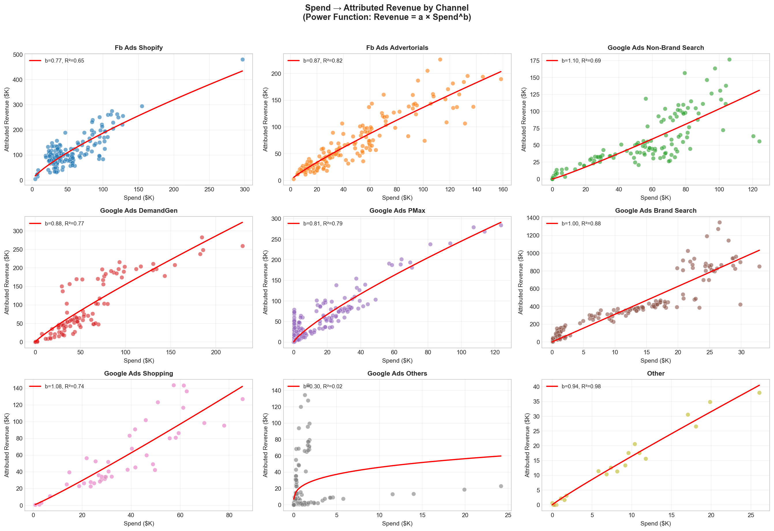
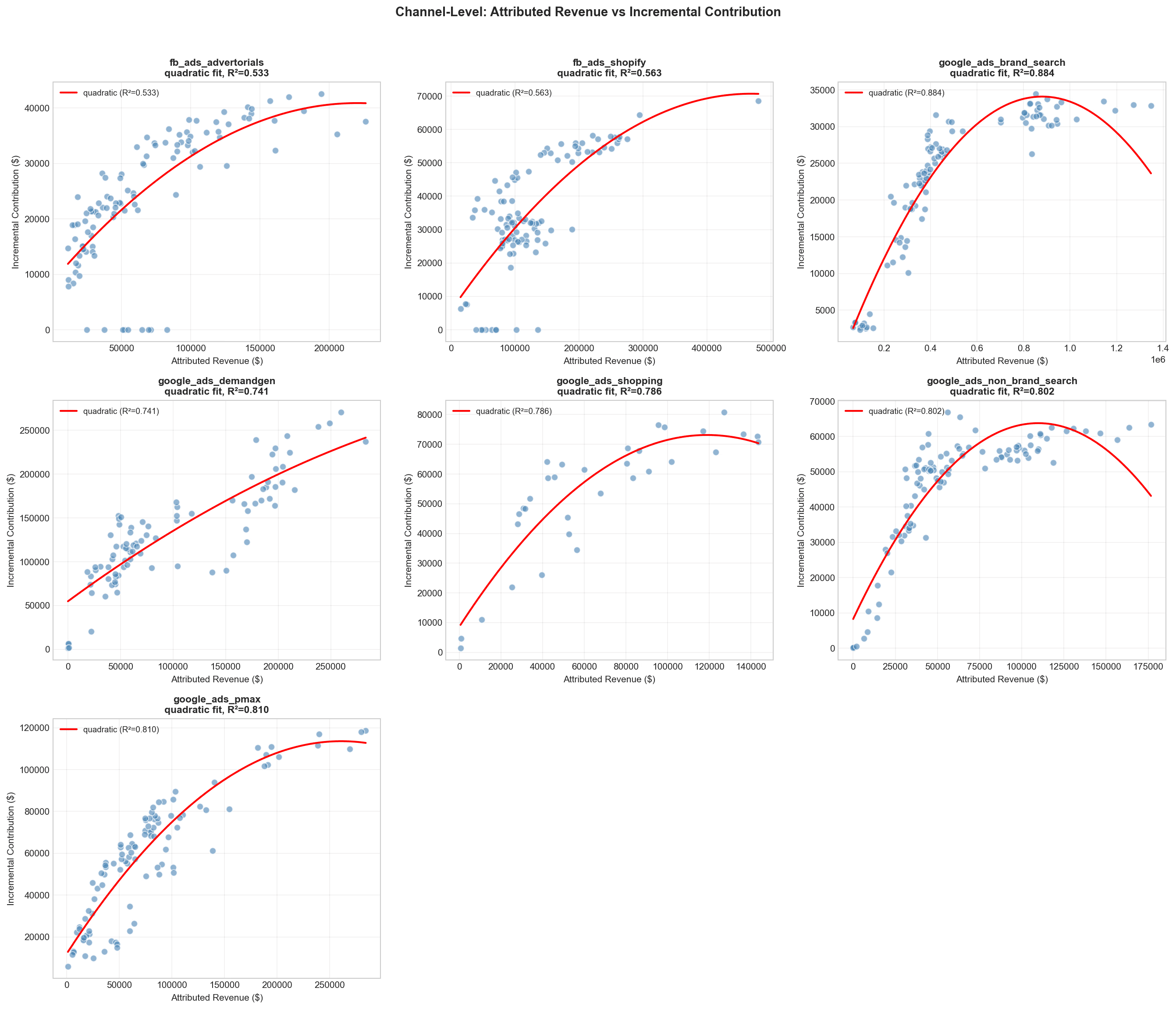
incrementality assessed by the MMM and the attribution:
incremental revenue = a * attribution ^ b
This step by step is better explained in this article, follow it step by step
If we see high R^2 between both relationship we can start attempting to distribute the incrementality at a campaign level.
Let's focus now at one campaign type: Meta Prospecting at €120K/month. Before going anywhere near campaign-level numbers, it is worth pinning down what each measurement system says at the channel-type level for this same period (t = last month).
One floor on what follows. The €156,000 channel-level incremental is itself a posterior with credible intervals — the MMM gives it as a distribution, not a point. Per-campaign iROAS reported to two decimals from a noisy top-line is spurious precision. Treat Rule B's output as a defensible distribution under stated assumptions, not as a 1.41× vs 1.29× difference that survives the underlying uncertainty.
Step 1 — What each measurement system reports at the channel level
Measurement system | Reported revenue from Meta Prospecting | Reported ROAS | What it actually measures |
|---|---|---|---|
Platform attribution (Meta-reported) | €432,800 | 3.61x | Conversions credited to a Meta touchpoint by the platform's attribution window — over-reported because the same user often sees the same conversion through multiple platforms. |
Marketing Mix Model (channel-level) | €156,000 | 1.30x | The incremental revenue Meta Prospecting genuinely caused, after netting out baseline demand, seasonality and the other channels — calibrated against geo-experiments where available. |
Gap (over-reporting ratio) | 2.77× | — | Platform attribution at this scale claims roughly 2.77× the revenue the MMM identifies as incremental. The €276,800 difference is the over-reporting we documented in Marketing Attribution Software Is Lying to You. |
The MMM gives one defensible number for the whole channel: €156,000 incremental. Platform attribution gives a per-campaign breakdown, but at an inflated level. Both are correct at the granularity each was designed for. Neither, on its own, answers the operational question.
Step 2 — The question for the rest of this section
We have €156,000 of incremental revenue earned by Meta Prospecting at t = last month. The channel contains four campaigns:
Campaign | Spend (€/mo) | Attributed Revenue | Attributed ROAS | Notes |
|---|---|---|---|---|
BFCM Creative Push | 48,000 | 220,800 | 4.60x | High-creative-rotation hero campaign |
Always-On Bestseller | 36,000 | 86,400 | 2.40x | Steady-state, mature creative |
Lookalike Test | 32,000 | 108,800 | 3.40x | Mid-spend test of new audience |
Long-Tail Interests | 4,000 | 16,800 | 4.20x | Small spend, long-tail audiences |
Channel total | 120,000 | 432,800 | 3.61x |
The question is: how do we distribute the €156K of channel-level incremental across these four campaigns? The two rules below answer it under different assumption sets.
Step 3 — Rule A applied: distribute by attributed share
Campaign | Attributed share of channel | Distributed incremental (€) | Distributed iROAS |
|---|---|---|---|
BFCM Creative Push | 51.0% | 79,560 | 1.66x |
Always-On Bestseller | 20.0% | 31,200 | 0.87x |
Lookalike Test | 25.1% | 39,156 | 1.22x |
Long-Tail Interests | 3.9% | 6,084 | 1.52x |
Total | 100% | 156,000 |
Rule A reports Long-Tail Interests at 1.52x distributed iROAS — better than the channel average. The signal is mechanically driven by attribution noise: €4K of spend earning a 4.20x attributed ROAS is one or two lucky high-AOV orders away from a phantom result.
Step 3.1 — Rule B Applied: distribute by spend × attributed-ROASβ
If we accept these assumptions:
Meta Prospecting campaigns share roughly the same diminishing-returns shape and adstock.
The remaining variance in attributed ROAS reflects creative and audience effects that spend alone does not capture, so its ranking is informative even though its magnitude is biased.
At very low spend, single-conversion noise dominates the weekly attributed ROAS — the 8-week trailing iROAS is what the rule should be read against, not the one-week number.
Then we use spend as the volume signal (linear) and attributed ROAS as the efficiency signal (compressed by β):
Weighti,t = Spendi,t × (Attributed_ROASi,t)β, with β ∈ [0, 1]; we use β = 0.3 in this example.
Plug the four campaigns in and read the result:
Campaign | Spend | Attr. ROAS | Weight (Spend × AR0.3) | Distributed € (rounded) | Distributed iROAS |
|---|---|---|---|---|---|
BFCM Creative Push | €48,000 | 4.60× | 75,870 | 67,621 | 1.41× |
Always-On Bestseller | €36,000 | 2.40× | 46,813 | 41,723 | 1.16× |
Lookalike Test | €32,000 | 3.40× | 46,195 | 41,172 | 1.29× |
Long-Tail Interests | €4,000 | 4.20× | 6,152 | 5,483 | 1.37× |
Total | €120,000 | 175,030 | 156,000 |
Two things are worth reading off this table.
The ranking matches attributed ROAS, exactly. BFCM (4.60×) at 1.41× distributed iROAS, then Long-Tail (4.20×) at 1.37×, then Lookalike (3.40×) at 1.29×, then Always-On (2.40×) at 1.16×. That is by construction — distributed iROASi ∝ Attributed_ROASiβ, so any monotonic compression of attributed ROAS preserves the ranking. The information in Rule B is the compression, not a re-ranking.
The compression is the value-add. Rule A spreads these four campaigns from 0.87× to 1.66× — a 0.79× range. Rule B compresses them to 1.16×–1.41× — a 0.25× range. Given that the channel-level MMM tells us attributed ROAS is over-reporting incremental impact by ~2.7× on average, the compression keeps the ranking signal while refusing to bet the budget on the magnitude signal. In practice this means smaller, more defensible reallocation moves than Rule A would suggest.
Long-Tail Interests at 1.37× distributed iROAS on €4,000 of spend deserves a note. The compression pulls its iROAS down from Rule A's 1.52× — which is helpful — but does not eliminate the underlying attribution noise: at €4K, a single high-AOV order moves attributed ROAS far more than creative effectiveness does. The protection is not the formula; it is the 8-week trailing iROAS, not the one-week snapshot.
Step 4 — Rule A vs Rule B at a glance
Same four campaigns, same €156,000 of channel-level incremental, two different distributions:
Campaign | Spend | Attr. ROAS | Rule A iROAS | Rule B iROAS | What changed |
|---|---|---|---|---|---|
BFCM Creative Push | €48K | 4.60× | 1.66× | 1.41× | Same leader, smaller margin. Rule B refuses to extrapolate from the highest attributed ROAS as if its full magnitude were causal. |
Always-On Bestseller | €36K | 2.40× | 0.87× | 1.16× | Rule A's spread punishes the workhorse below break-even on the strength of low attributed ROAS alone. Rule B compresses the gap and the workhorse looks viable. |
Lookalike Test | €32K | 3.40× | 1.22× | 1.29× | Both rules agree directionally; the compression nudges efficiency upward by trusting the ranking more than the magnitude. |
Long-Tail Interests | €4K | 4.20× | 1.52× | 1.37× | Rule B compresses the low-spend noise but does not eliminate it. The 8-week trailing iROAS is what filters single-conversion outliers, not the formula. |
And the rules themselves, side by side:
Rule A — Attributed Share | Rule B — Spend × Attr-ROASβ, β = 0.3 | |
|---|---|---|
What it does | Splits the channel-level incremental in proportion to each campaign's share of attributed revenue inside the channel. | Splits the channel-level incremental by spend (linear) weighted by attributed ROAS raised to a sub-linear power. Preserves Rule A's ranking; compresses its magnitudes. |
Inputs needed per period | Attributed revenue per campaign. | Spend AND attributed ROAS per campaign. |
Who wins (the bias) | Campaigns with high attributed ROAS at low spend — the small-numbers bias rewards single-conversion noise. | Same ranking as Rule A: campaigns with higher attributed ROAS earn more credit per euro of spend. The difference is that the gap is compressed, so the high-attributed-ROAS leader absorbs less of the channel's incremental than under Rule A. |
Failure mode | A €500/mo campaign with one lucky high-AOV order claims an outsized slice of channel-level incremental. | Same small-numbers bias as Rule A at very low spend, in compressed form. The 8-week trailing iROAS, not the weekly snapshot, is the operational filter. |
Use when | Quick first-pass cut, low-stakes reporting, accounts with little attribution-noise asymmetry. | Production weekly reallocation calls; whenever attributed ROAS magnitudes are likely over-reported (almost always in performance media) and you want defensible compression rather than the raw spread. |
Directional output for this account | Says BFCM is the hero at 1.66× and the workhorse Always-On is below break-even at 0.87×. The first claim over-extrapolates, the second is wrong. | Same ranking as Rule A: BFCM > Long-Tail > Lookalike > Always-On. Compresses the spread from Rule A's 0.87×–1.66× to 1.16×–1.41×: the hero looks less heroic, the workhorse looks viable, and the gaps are small enough that the 8-week trailing average — not a single week — should drive scale/hold decisions. |
Step 5 — Read the output: what to do this week
Campaign | Distributed iROAS | Action |
|---|---|---|
BFCM Creative Push | 1.41× | Hold or carefully scale — leading the channel after compression, but the gap over peers is small (0.04× over Long-Tail, 0.12× over Lookalike). Confirm against the 8-week trailing average before adding budget. |
Long-Tail Interests | 1.37× | Investigate, don't scale yet — at €4K of spend a one-week iROAS is dominated by individual conversions. Compression brought it down from Rule A's 1.52× but didn't eliminate the noise. Confirm against the 8-week trailing average; if it sustains above 1.30× there, treat it as a creative/audience signal worth scaling gradually. |
Lookalike Test | 1.29× | Hold; consider scaling if BFCM shows fatigue — outperforming Always-On but trailing the leaders. The compressed spread does not justify a reallocation away from BFCM on a single week's data. |
Always-On Bestseller | 1.16× | Hold — the lowest distributed iROAS in the channel, but Rule B's compression rescues it from Rule A's 0.87× phantom verdict. Productive at current spend; no headroom for additional budget. |
A "kill" rarely comes from this rule alone. Kills should come from creative fatigue, audience exhaustion, or cohort-quality drops — not from a one-week distribution number. Use the 8-week trailing iROAS, not the weekly snapshot, for scale and retire decisions.
Why 8 weeks? Long enough to wash out single-conversion noise on small campaigns and one full creative-fatigue cycle (typically 2–6 weeks for performance creatives), short enough that an 8-week-old observation still reflects the current creative and audience mix. Shorter windows (e.g. 4 weeks) keep more signal but stay too noisy for low-spend campaigns; longer windows (12+ weeks) over-smooth through creative refreshes and seasonal pivots and stop being predictive.
How to know the rule has broken for an account. Three signals to watch: (1) a small campaign repeatedly winning the weekly iROAS leaderboard while its 8-week trailing average sits much lower — single-conversion noise is the driver, not creative effectiveness; (2) pausing the highest-distributed-iROAS campaign for a week and channel-level revenue holds — attributed ROAS was capturing audience overlap, not creative effectiveness; (3) a single campaign's weekly iROAS diverging from its 8-week trailing average by more than 30% for two consecutive weeks — the underlying creative, audience or offer has shifted and the assumptions no longer hold for that campaign.
Step by step campaign
The rule is intended to support, not replace, the weekly within-channel reallocation conversation. A typical use:
The MMM produces channel-level incremental revenue per period (for example, €156,000 for Meta Prospecting last week).
Map relationship between incrementality and attribution and spend - formula here
Rule B distributes that figure across all active campaigns in the channel for the same period.
Do this daily or weekly.
The rule is a structured procedure that produces a number from inputs (channel-level incremental from the MMM, campaign-level spend and attributed ROAS from the platform) and a fixed parameter set (β = 0.3) that is held constant within a quarter. It is not a causal measurement. Where the assumptions hold for a given account, the rule's output is the defensible distribution of channel-level incrementality across campaigns in that account; where the assumptions fail, the falsifiability tests above describe how to detect it.
This article is part of a series on incrementality measurement. Prior pieces: The Incrementality Multiplier Is Broken and Marketing Attribution Software Is Lying to You: 792-Model Proof.
Methodology references: 792 MMM models, 194 advertisers, 2017–2025 substrate. Distribution rule fitted against the channel-level decompositions of that substrate. The β = 0.3 default is the cross-validated median across the book; client-specific calibration available on request.
Author: Gabriele Franco, Founder & CEO of Cassandra
Frequently Asked Questions
Why can't I measure campaign-level incrementality directly from an MMM?
Three compounding reasons. First, statistical power: a single campaign at 5–15% of channel spend generates too little revenue variation to rise above the model's noise floor. Second, multicollinearity: campaigns inside the same channel respond to the same external triggers simultaneously, so the model cannot separate their individual contributions. Third, consistency: most campaigns run for 2–6 weeks and are then paused or retired — not long enough to estimate a stable coefficient. Any one of these reasons alone blocks causal identification at campaign level.
Does this method work without running holdout tests for every campaign?
Yes. Rule B only requires two inputs per campaign per week: spend and attributed ROAS from your platform reports. The channel-level incremental revenue comes from your existing MMM. No additional holdout tests are needed to apply the distribution rule — the entire method runs on data your team already has access to.
What is the difference between Rule A and Rule B?
Rule A splits channel-level incremental revenue in proportion to each campaign's share of attributed revenue inside the channel. It is simple but biased toward small campaigns with single-conversion noise. Rule B weights campaigns by spend × attributed ROAS, with both signals compressed by the same exponent (β = 0.3), so neither dominates. Rule B is recommended for any reallocation decision that will actually move budget.
What is the β parameter in Rule B and how do I set it?
β is the exponent applied to attributed ROAS in the weighting formula Weight = Spend × Attr_ROASβ. Spend enters linearly; attributed ROAS is dampened by β. β must lie in the [0, 1] interval — β = 0 ignores attributed ROAS entirely and Rule B becomes "split by spend share." β = 1 removes the dampening and the formula reduces to spend × attributed ROAS, which is attributed revenue, exactly Rule A. Values between trade off "trust spend share" against "trust attributed ROAS as-is". The default used in this example is β = 0.3, chosen to produce stable campaign-level rankings across approximately 200 channel-level MMM decompositions in the Cassandra book — i.e., the rule's output is robust to small perturbations of the inputs. This is rank-stability, not causal ground truth (there is no campaign-level ground truth). Start at 0.3 and adjust only if you have a specific calibration reason.
How often should I recompute the campaign-level incrementality distribution?
Weekly, using the same period as your MMM refresh cycle. Build the monitoring table on a rolling basis and use the 8-week trailing iROAS as the primary signal for scale/hold decisions — single-week snapshots are too noisy to act on alone. If a campaign's weekly iROAS diverges from its 8-week trailing average by more than 30% for two consecutive weeks, treat that as an investigation trigger, not an immediate scaling decision.